


Capabilities
DNA Is Our Foundation
Providing cancer researchers with the only single-cell technology that simultaneously measures single nucleotide variation (SNV), copy number variation (CNV), and protein data from the same cells. Our multi-omics platform connects genotype and phenotype in each cell, dissecting the architecture of tumors with unprecedented resolution.
Single-cell Genomics (DNA)
SNV
Leverage single-cell technology to detect rare clonal populations and identify co-occurrence and zygosity.
SNV + CNV
Characterize genetic and copy number aberrations using a single comprehensive platform.
Single-cell Multi-omics (DNA + Protein)
DNA + Protein
Gain a true multi-omics picture from genotype to phenotype.
Applications
Products
The Tapestri Platform
The first and only single-cell technology developed to reveal biomarkers that help stratify patients, signal resistance, and predict relapse. Tapestri’s powerful multi-omics capability — connecting genotype and phenotype — opens the door to a deeper understanding and improved treatment of cancer.
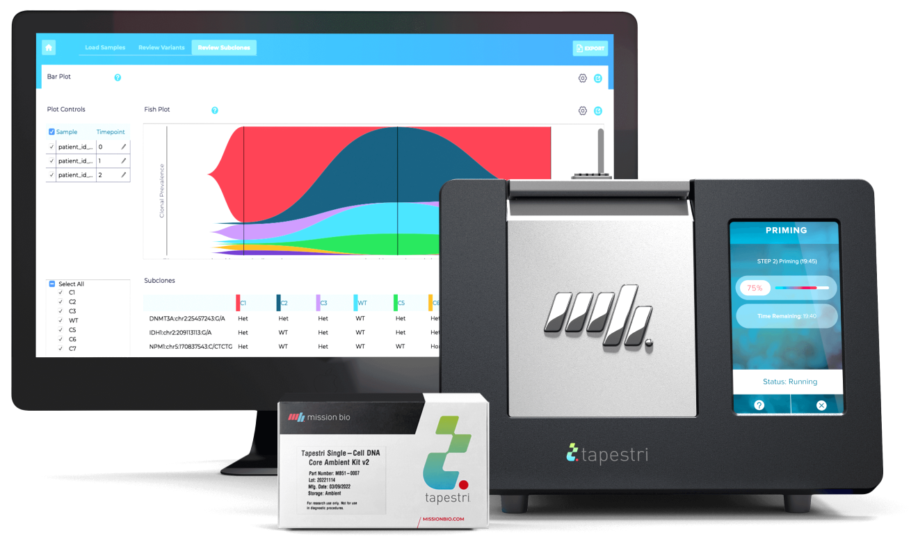
Tapestri Platform
An end-to-end workflow from sample preparation to visualization with publication-ready insights for single-cell sequencing analysis.
Panels
Targeted panels provide focus on key regions of interest for efficient use of sequencing budget and analysis time.
News


